Builder Functions & Interface Overview
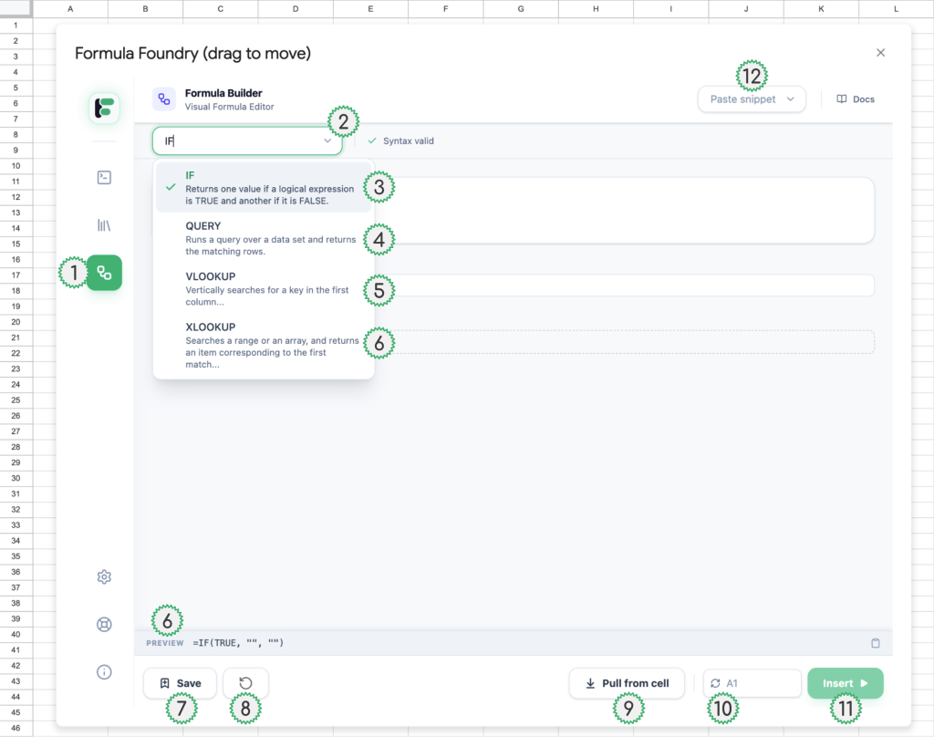
- Navigation to Visual Formula Builder feature
- Dropdown to select type of formula / function the Visual Formula Builder will create
- Select to build IF statement formulas
- Select to build QUERY statement formulas
- Select to build VLOOKUP statement formulas
- Select to build XLOOKUP statement formulas
- Save a formula created in the Visual Formula Builder as a Snippet (in the Snippet Library feature)
- Reset / clear the Visual Formula Builder entry fields
- Pull the formula from the currently selected cell in your sheet
- NOTE: when pulling in an existing formula, make sure the Visual Formula Builder has the same type of formula function selected in its dropdown the formula in the cell you are pulling in — E.g., IF, QUERY, VLOOKUP, XLOOKUP)
- Currently selected cell in Sheet
- Displays the name of the cell currently synced with the Editor
- Sync (refresh icon) button updates which cell is currently selected in the sheet
- Insert Editor code (of the currently viewed tab) into the currently synced cell in the sheet
IF Statements Interface
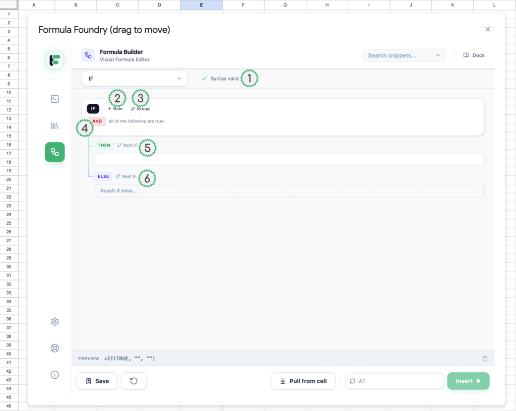
- Indicates the syntax of the formula built is valid, and not containing any issues or missing parts (when there is an issue, this text changes to “Syntax error”
- Click to add a rule to your IF statment
- Click to add a group to your IF statment, which can contain multiple rules sharing the same initial condition
- Click to switch between AND or OR
- Expand and collapse adding additional conditions to ‘THEN’ statement
- Expand and collapse adding additional conditions to ‘ELSE’ statement
IF Statements Interface Continued
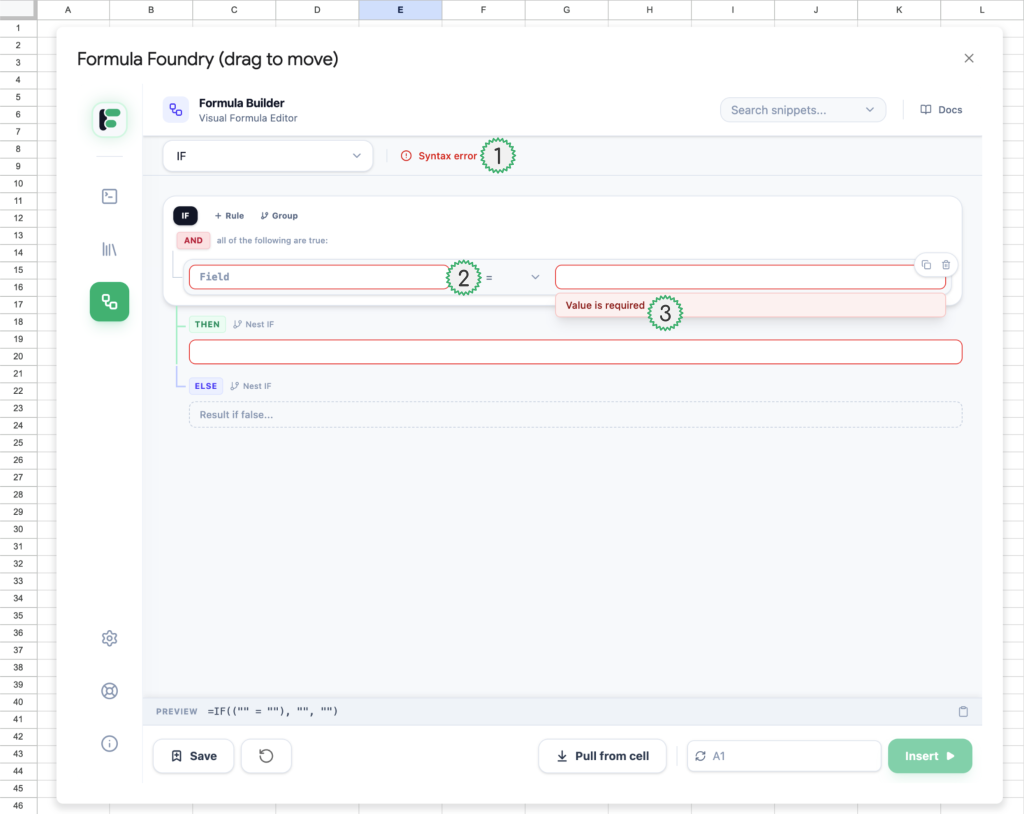
- Indicates the syntax of the formula built is not valid, and containing issues or missing parts (when there isn’t an issue, this text changes to “Syntax valid”
- Fields highlighted in red require attention, either:
- No value is present in a required field for the formula to funtion
- A value has an incorrect format for the field
- Additional context for entry field errors are provided in mini pop-ups, when the user has their cursor active in a cell
IF Statements Interface Continued
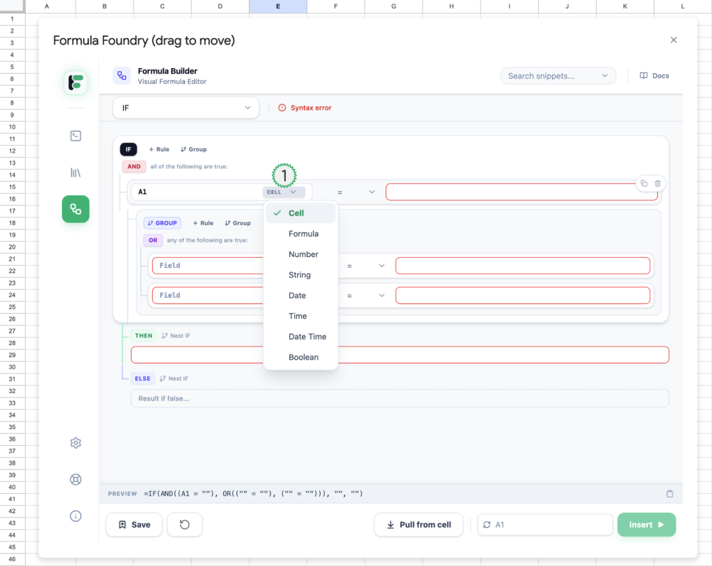
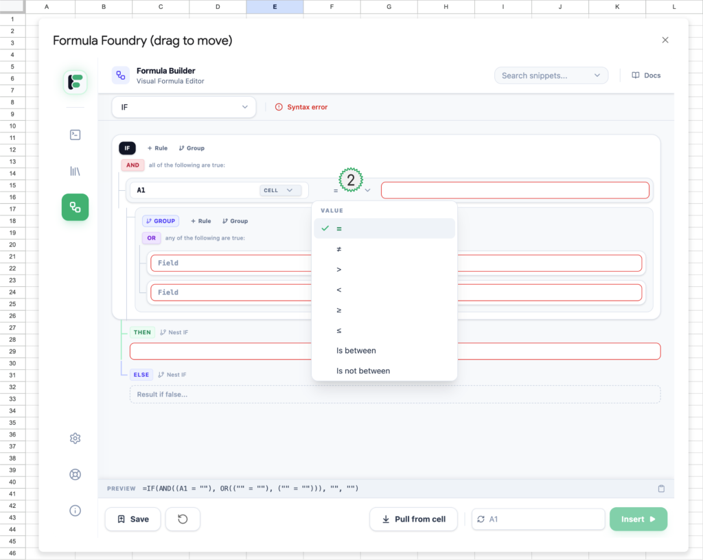
- Formula Foundry will auto-detect and set the value type, based on the entry from the user, BUT users can also manual edit/set what type of input is in place by using the this dropdown — options:
- Cell
- Formula
- Number
- String
- Date
- Time
- Date Time
- Boolean
- User must set the relationship between values
- Equals
- Does Not Equal
- Greater Than
- Less Than
- Greater Than or Equal To
- Less Than or Equal To
- Is Between
- Is Not Between
QUERY Interface
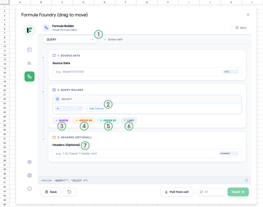
- QUERY selected as type of formula / function the Visual Formula Builder will create
- Add Columns to selection included in QUERY
- Include “Where” conditions to QUERY
(see expanded appearance of this interface in next annotated screen) - Include “Group By” conditions to QUERY
(see expanded appearance of this interface in next annotated screen) - Include “Order By” conditions to QUERY
(see expanded appearance of this interface in next annotated screen) - Include “Limit” conditions to QUERY
(see expanded appearance of this interface in next annotated screen) - Include “Header” conditions to QUERY
(see expanded appearance of this interface in next annotated screen)
QUERY Interface Continued
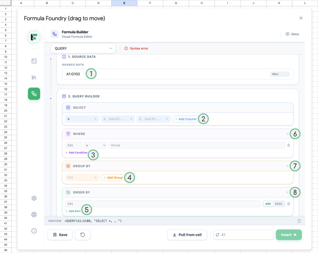
- Add / set Source Data (array) that the QUERY will reference
- This is the specific range of cells, named range, or array that contains the raw information you want to analyze. It acts as the “database” that the formula reads from.
- Key characteristic: The QUERY function does not change this data; it only reads it to generate a new result elsewhere.
- Formatting: It can be a direct reference (e.g., ‘Sheet1’!A1:Z100), a Named Range (e.g., SalesData), or even the result of another formula.
- This is the specific range of cells, named range, or array that contains the raw information you want to analyze. It acts as the “database” that the formula reads from.
- Expanded appearance of “Column” conditions
- (Select) This clause determines exactly which columns from your Source Data will be displayed in the final output.
- Function: If you omit this clause, the formula returns all columns (like Select *). If you specify columns (e.g., Select A, C), it returns only those specific ones, in the order you list them.
- (Select) This clause determines exactly which columns from your Source Data will be displayed in the final output.
- Expanded appearance of “Where” conditions
- This is your filter. It tells the formula to only return rows that meet specific criteria (e.g., “Where B > 100” or “Where C contains ‘Completed'”).
- Expanded appearance of “Group By” conditions
- This aggregates your data, functioning similarly to a Pivot Table. It groups rows that have the same value in a specified column so you can perform calculations on them (like summing or counting) to get a single result for that group.
- Expanded appearance of “Order By” conditions
- This sorts your results. You specify which column to sort by and the direction: asc (ascending, default) or desc (descending).
- Close / remove of “Where” conditions
- Close / remove of “Group By” conditions
- Close / remove of “Order By” conditions
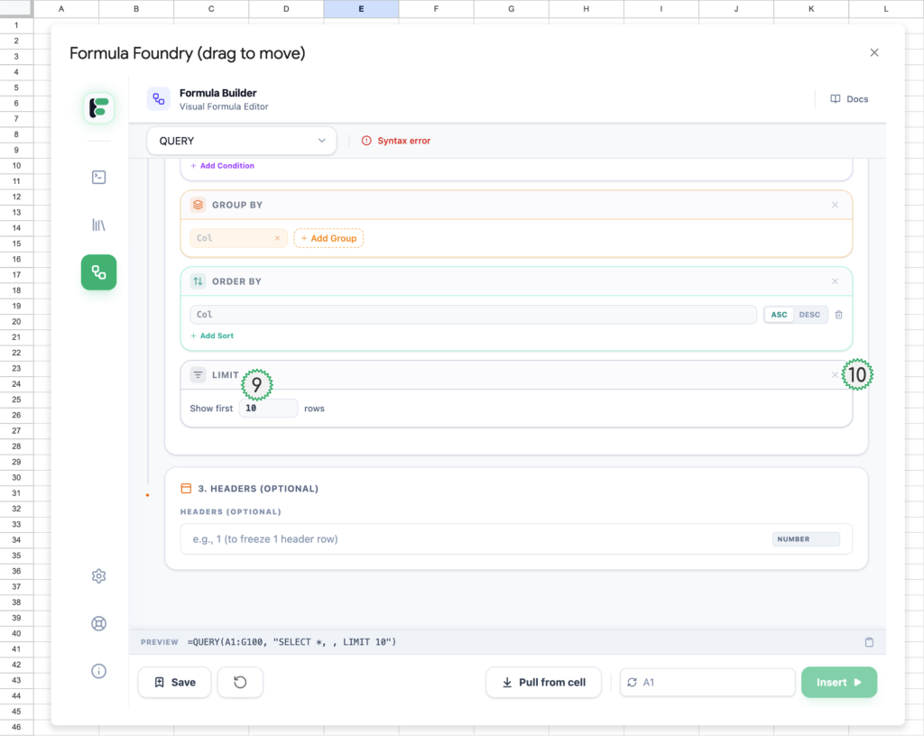
- Expanded appearance of “Limit” conditions
- This restricts the number of rows returned. It is often used with Order By to find “Top X” or “Bottom X” results (e.g., “Order by D desc Limit 5” gives you the top 5 highest values).
- Close / remove of “Limit” conditions
VLOOKUP Interface
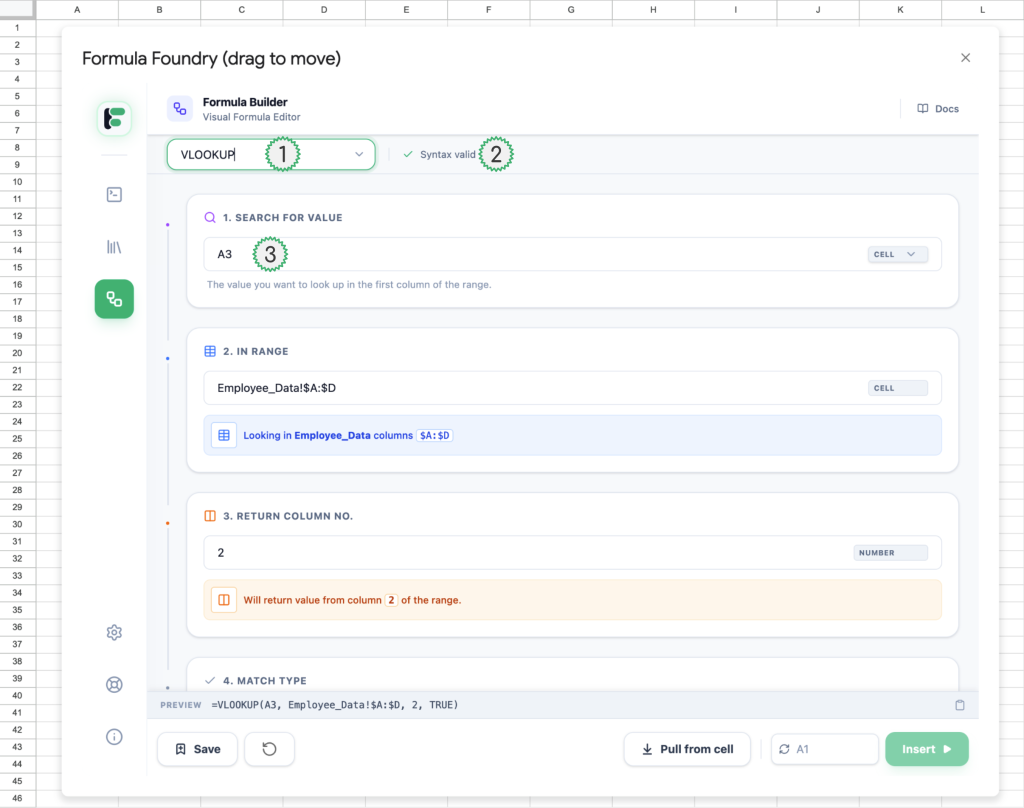
- VLOOKUP selected as type of formula / function the Visual Formula Builder will create
- Indicates the syntax of the formula built is valid, and not containing any issues or missing parts (when there is an issue, this text changes to “Syntax error”)
- Add / set the Lookup Value VLOOKUP will be looking / searching for
- (lookup_value) The specific value or cell reference you want to find. VLOOKUP always looks for this value in the first (leftmost) column of the range you select.
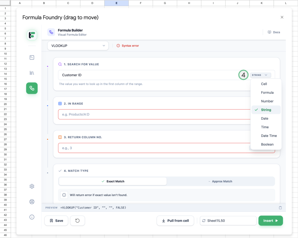
- Formula Foundry will auto-detect and set the value type, based on the entry from the user, BUT users can also manual edit/set what type of input is in place by using the this dropdown — options:
- Cell
- Formula
- Number
- String
- Date
- Time
- Date Time
- Boolean
VLOOKUP Interface Continued
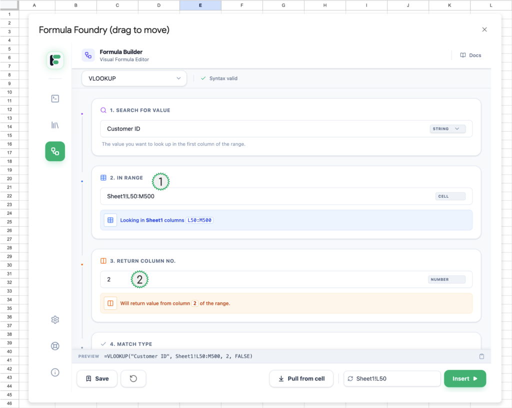
- Add / set Range (array) that the VLOOKUP will reference
- (table_array) The entire block of data you want the formula to consider. This range must include both the column with the “Search Key” (which must be column 1) and the column containing the “Result.”
- Add / set Return Column that the VLOOKUP will reference
- (col_index_num) The column number within your Range that contains the data you want to get back.
- Example: If your Range is A:C, Column A is 1, Column B is 2, and Column C is 3.
- (col_index_num) The column number within your Range that contains the data you want to get back.
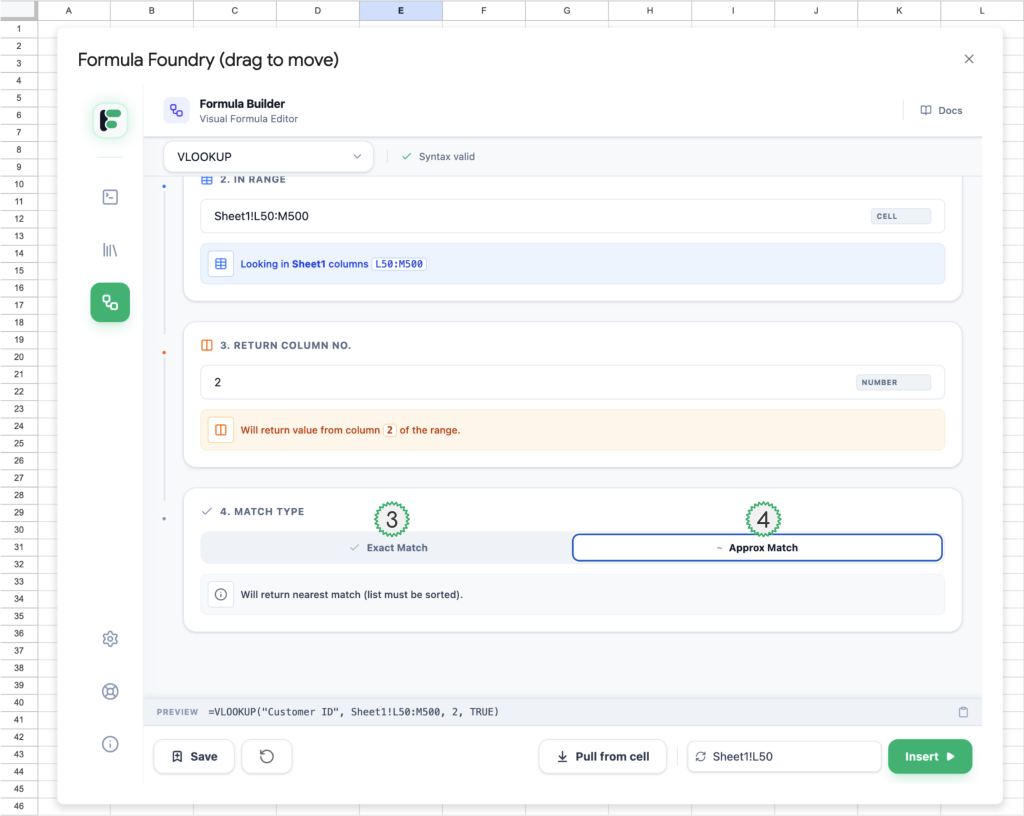
- Define Match Type:
- Exact Match
- (FALSE or 0) The function searches for a value identical to the “Search for Value.” If it doesn’t find it, it returns an error (#N/A). This is the most common setting for looking up specific IDs or names.
- Approximate Match
- (TRUE or 1 or omitted) If an exact match isn’t found, the function returns the next largest value that is less than your search value.
- Critical Note: For this to work correctly, the first column of your Range must be sorted in ascending order.
- (TRUE or 1 or omitted) If an exact match isn’t found, the function returns the next largest value that is less than your search value.
- Exact Match
XLOOKUP Interface
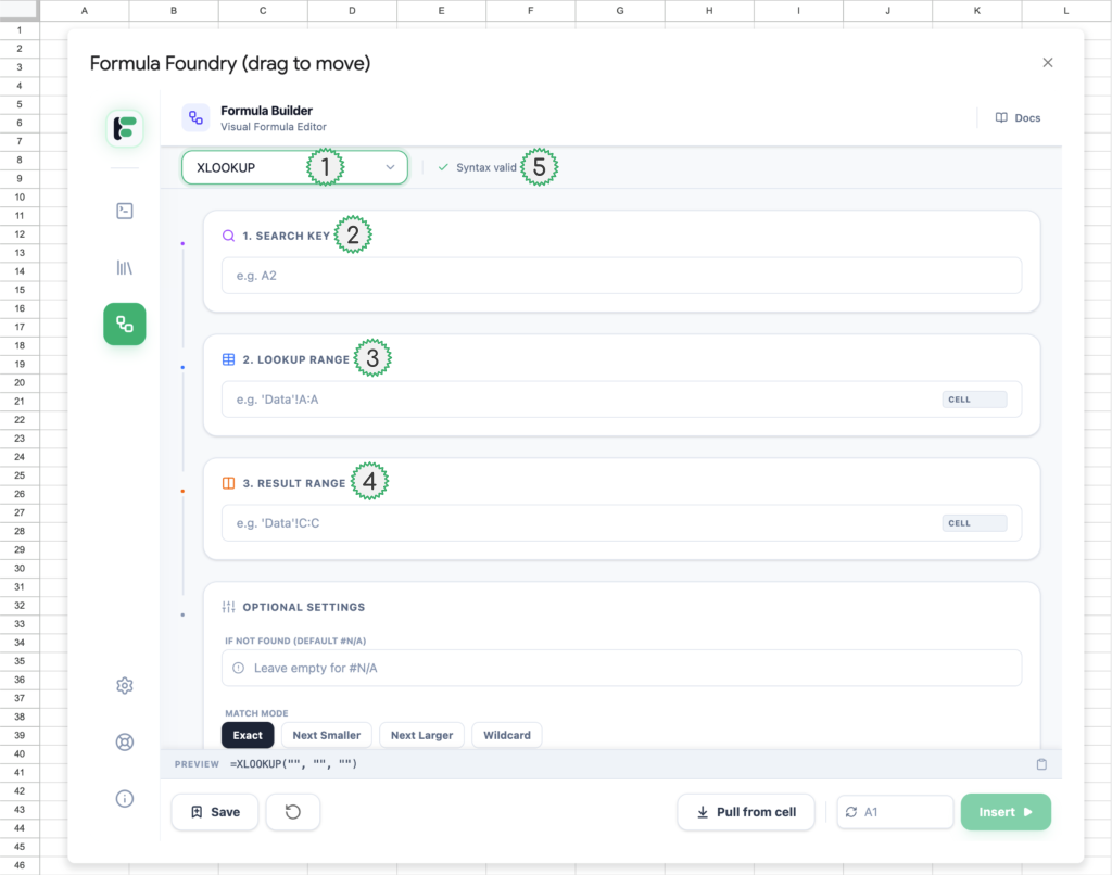
- XLOOKUP selected as type of formula / function the Visual Formula Builder will create
- Add / set Search Key
- (lookup_value) The specific value, text, or cell reference you want to find. This is the “target” you are looking for.
- Add / set Lookup Range
- (lookup_array) The specific column or row where XLOOKUP should search for the Search Key.
- Add / set Result Range
- (return_array) The column or row that contains the value you want returned. It must correspond in size to the Lookup Range (e.g., if the lookup range is rows 1–10, the result range must also be rows 1–10).
- Indicates the syntax of the formula built is valid, and not containing any issues or missing parts (when there is an issue, this text changes to “Syntax error”)
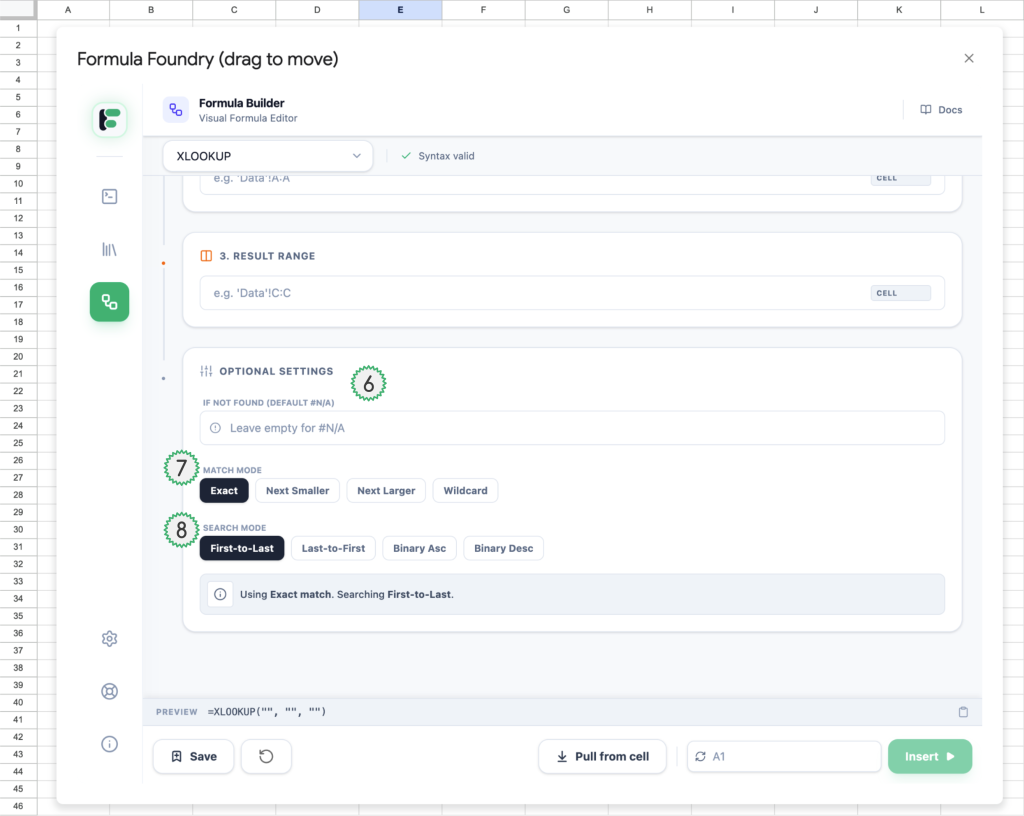
- Optional Settings to include in XLOOKUP conditions
- Match Mode
- Exact
- (0) The default setting. The function searches for a value that is identical to the Search Key. If it doesn’t find it, it returns an error (N/A).
- Next Smaller
- (-1) Searches for an exact match first. If none is found, it returns the next smaller value (the closest value that is less than the Search Key).
- Next Larger
- (1) Searches for an exact match first. If none is found, it returns the next larger value (the closest value that is greater than the Search Key).
- Wildcard
- (2) Allows the use of wildcard characters in your Search Key.
- represents any sequence of characters.
- ? represents any single character.
- (2) Allows the use of wildcard characters in your Search Key.
- Exact
- Search Mode
- First-to-last
- (1) The default setting. It starts at the top (or left) of the Lookup Range and moves down (or right), stopping at the first match it finds.
- Last-to-first
- (-1) Starts at the bottom (or right) of the Lookup Range and moves up (or left). This is useful for finding the most recent entry in a chronological list.
- Binary Asc
- (2) Performs a binary search on data sorted in ascending order (A-Z or 1-10). This is significantly faster on massive datasets but returns errors if the data isn’t sorted correctly.
- Binary Desc
- (-2) Performs a binary search on data sorted in descending order (Z-A or 10-1). Like above, this is for speed but requires correctly sorted data.
- First-to-last
- Match Mode
Was this article helpful?
Thanks for your feedback!